May 26th 2015, GPS Signal Distribution
← May 25th 2015 Weighted Least Squares | ● | May 26th 2015 Application of Least Squares to GPS →
With the GPS accuracy describing a confidence interval of 50%, the coordinates of a GPS measurement $m_i$ of a non-moving receiver should be distributed normally under the Gaussian distribution function $\Phi(x)$.
Not exactly. Since we are in 3D space, the coordinates are not statistically independent, so the distribution is not Gaussian, but rather circular Gaussian (or Rayleigh-distributed). Still not exactly. In experiments the real-world distribution shows to be log-normal (see here for a comparison).
For our purposes, however, we project the distribution onto a vertical plane parallel to the trajectory of the receiver. In this case the projections can be considered to be distributed normally on the trajectory plane. For a variance of $\sigma$ and an estimated mean of $\mu=0$ the Gaussian normal distribution is
A confidence interval of 50% for a particular accuracy $a$ means that
For a given accuracy $a$, the variance $\sigma$ of the corresponding probability distribution is
So the distribution function of the GPS measurements is the following:
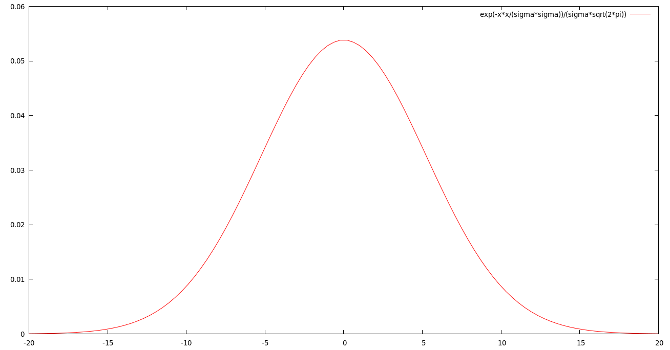
Here is an example distribution for $a = 5m$ accuracy projected on the trajectory plane (and plotted with gnuplot):
gnuplot> sigma = 5 * 1.4826
gnuplot> plot [-20:20] exp(-x*x/(sigma*sigma))/(sigma*sqrt(2*pi))
← May 25th 2015 Weighted Least Squares | ● | May 26th 2015 Application of Least Squares to GPS →